FHKN

Fourier-Hermite Kinetic Network for Rarefied Gas Transport

PyTorch Kinetic Networks Porous Media GPU
FHKN Prediction Results

Predicting Steady-State Gas Transport from Early Transients

Transient to
Steady State

Simulating gas transport in nanoporous shale via the Lattice Boltzmann Method (LBM) requires up to 300,000 iterations to converge—a severe computational bottleneck. FHKN bypasses this by learning a direct mapping from the first ~600 early transient iterations to the final steady-state velocity field.

The network is trained on distribution functions $f_i(\mathbf{x}, t)$ from simple random geometries and generalizes zero-shot to complex, highly tortuous porous media at up to 4× the training resolution.
Key Results

  • Accuracy ($R^2$): ≥ 0.90
  • Optimal Input: $N = 600$ iters
  • Super-resolution: 4× Zero-shot
  • GPU Speedup: 10–1000×
  • Permeability Error: < 10%

01. Training Data
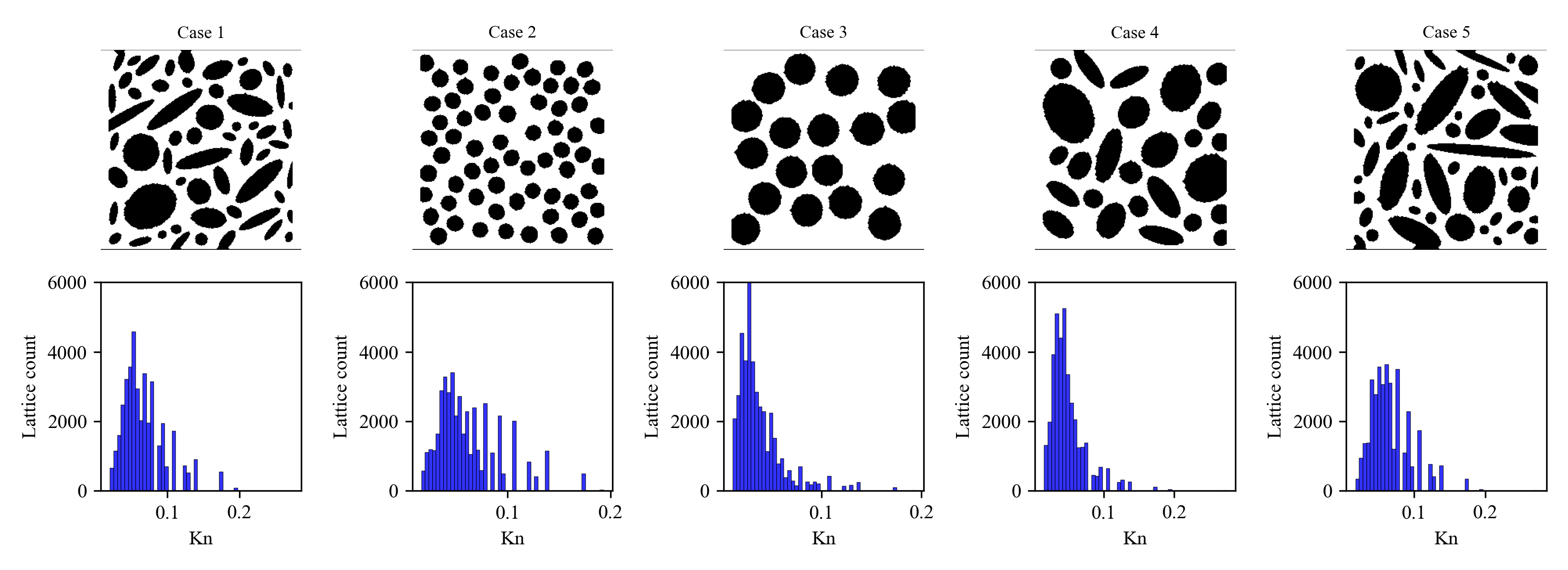
FHKN training cases: pore geometries and Knudsen number distributions

Training cases: pore structure (top) and local Knudsen number (bottom)

Five Synthetic Geometries

Five $256\times256$ pore geometries were generated by randomly placing circular and elliptical obstacles. Methane transport was simulated at $2\,\mathrm{MPa}$ and $300\,\mathrm{K}$ using an optimized C++ MRT-LBM solver.

The local Knudsen number ranges from 0.02–0.2, spanning the slip and transitional flow regimes where rarefaction is significant. The network input is a tensor $\mathbf{f} \in \mathbb{R}^{9 \times T}$ of $D_2Q_9$ distribution functions over a temporal window of length $T$. The target output is the steady-state velocity field $[\hat{u}_x, \hat{u}_y]$.

Cases 1–2 (82,511 cells) form the training set. Cases 3–5 serve as the test set on unseen geometries.

02. Network Architecture
FHKN Architecture Diagram

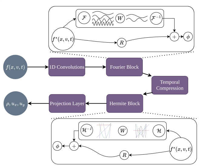
FHKN architecture: temporal lifting → Fourier blocks → Hermite stage → MLP

Three-Stage Design

The architecture is physically motivated by the structure of the Boltzmann equation. Each stage maps to a distinct aspect of kinetic theory.

  • Stage 1 — Temporal Lifting: 1D convolutions extract short-range transient features from the 9-channel population sequence.
  • Stage 2 — Fourier Spectral Blocks: Channel mixing in the frequency domain captures long-range relaxation dynamics.
  • Stage 3 — Hermite Reconstruction: Projects features onto $D_2Q_9$ Hermite basis moments, aligning with the macroscopic Navier-Stokes limit.

Fourier Spectral Block

Within each spectral block, a learned complex-valued channel-mixing matrix $W(k)$ is applied to the lowest $K$ Fourier modes. Frequencies $k \ge K$ are zeroed out (low-pass kinetic filter). A pointwise residual pathway $R(t)$ is added before the nonlinearity:

Hermite Reconstruction Stage

After temporal aggregation, the feature vector is projected onto Hermite polynomials up to second order ($H_0, H_1^\alpha, H_2^{\alpha\beta}$), generating moments corresponding to density and momentum. Learnable coefficients $\omega$ rescale each moment, and a parameterized residual $\gamma_i s_i$ is added:

This mathematically mirrors the Gauss–Hermite quadrature underlying LBM — discarding high-frequency kinetic noise and mapping directly to macroscopic velocity.

03. Results
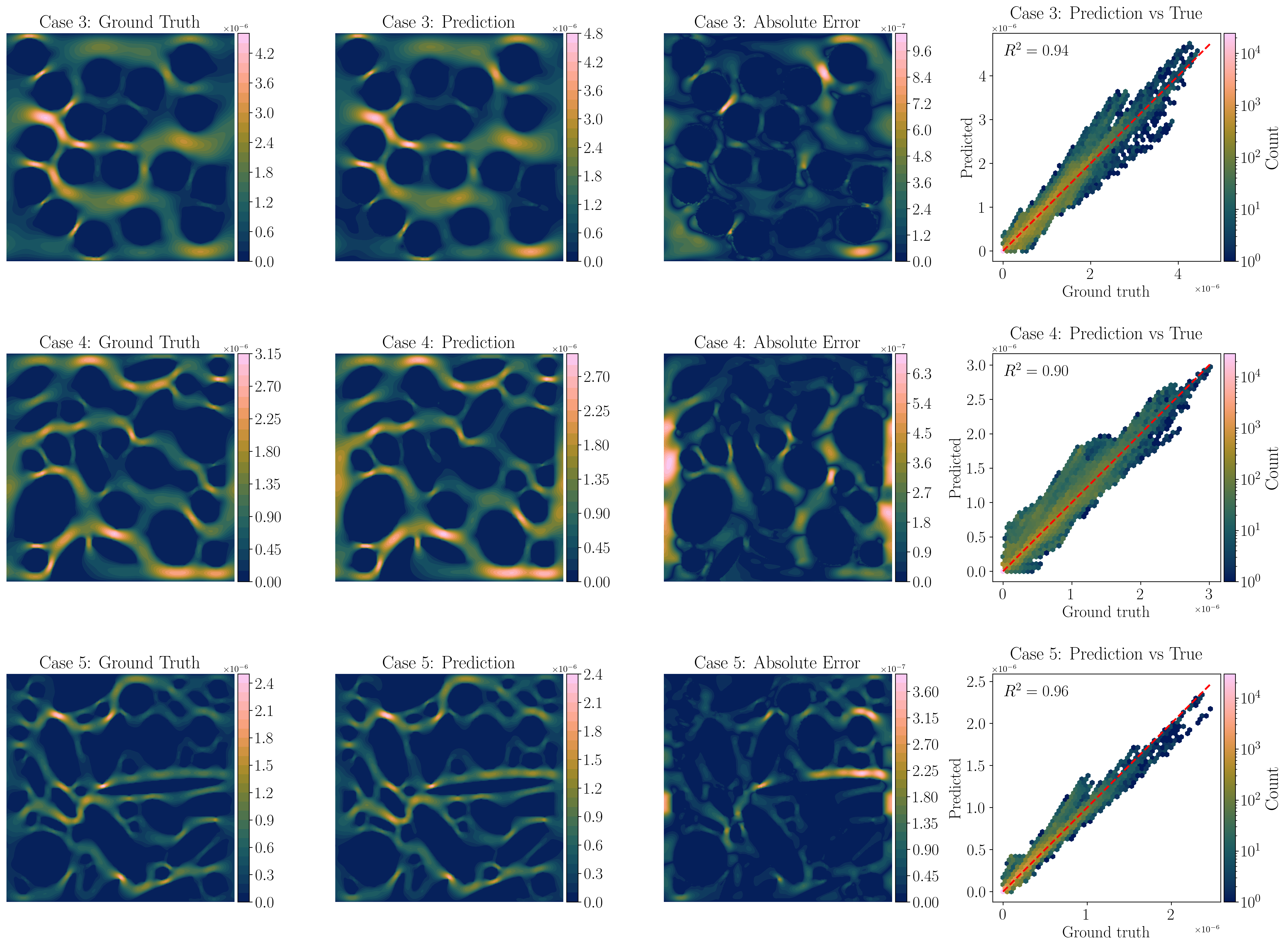
FHKN prediction vs LBM ground truth for cases 3, 4, 5

Left to right: LBM ground truth · FHKN prediction · absolute error · scatter ($R^2$) — for test cases 3, 4, 5

Model Comparison: FN vs FHKN vs HN

FHKN consistently outperforms isolated Fourier (FN) and Hermite (HN) networks across all tested resolutions ($256^2$, $512^2$, $1024^2$), while maintaining near-identical accuracy from training resolution up to 4× finer grids — a zero-shot super-resolution capability.

Resolution Metric FN FHKN HN
256 × 256 (Training) Avg $R^2$ 0.910 0.933 0.913
Avg Rel. $L_2$ 0.177 0.157 0.170
512 × 512 Avg $R^2$ 0.910 0.933 0.910
Avg Rel. $L_2$ 0.183 0.160 0.173
1024 × 1024 (4× Super-res) Avg $R^2$ 0.910 0.927 0.913
Avg Rel. $L_2$ 0.193 0.170 0.183
04. Blind Tests

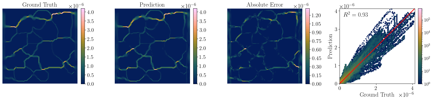
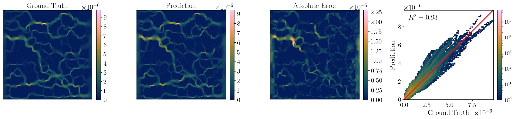
To rigorously test generalization, two highly tortuous $1024 \times 1024$ porous domains were generated from random Gaussian noise — geometries never seen during training with substantially higher topological complexity. The LBM solver required 300,000 iterations for Case 1 and 66,000 iterations for Case 2 to converge. FHKN used only the first 2,400 transient iterations as input.

FHKN blind test 1 prediction

Blind Test 1 — $R^2 = 0.93$

FHKN blind test 2 prediction

Blind Test 2 — $R^2 = 0.93$

Permeability Prediction

Extracting permeability directly from the early-transient LBM (the raw network input) gives 20% and 15% error for the two cases. FHKN reduces these to 6% and 9%, successfully mapping the early transient to the steady-state limit.

LBM Transient LBM Steady (GT) FHKN Error (FHKN) Error (Transient)
Case 1 3.147e-19 m² 2.602e-19 m² 2.764e-19 m² 6.2% 20.7%
Case 2 6.612e-19 m² 5.730e-19 m² 6.255e-19 m² 9.2% 15.4%

Publication & Source Code

Fourier-Hermite Kinetic Network for Gas Transport under High Knudsen Numbers

Rustamov, N. & Aryana, S. A.

Paper currently under review at InterPore Journal. Publication, dataset, and source code will be posted upon acceptance.


← Back to Projects